
Multimodal Imaging of Pressed Seaweed: RGB, Hyperspectral and XRF Fusion
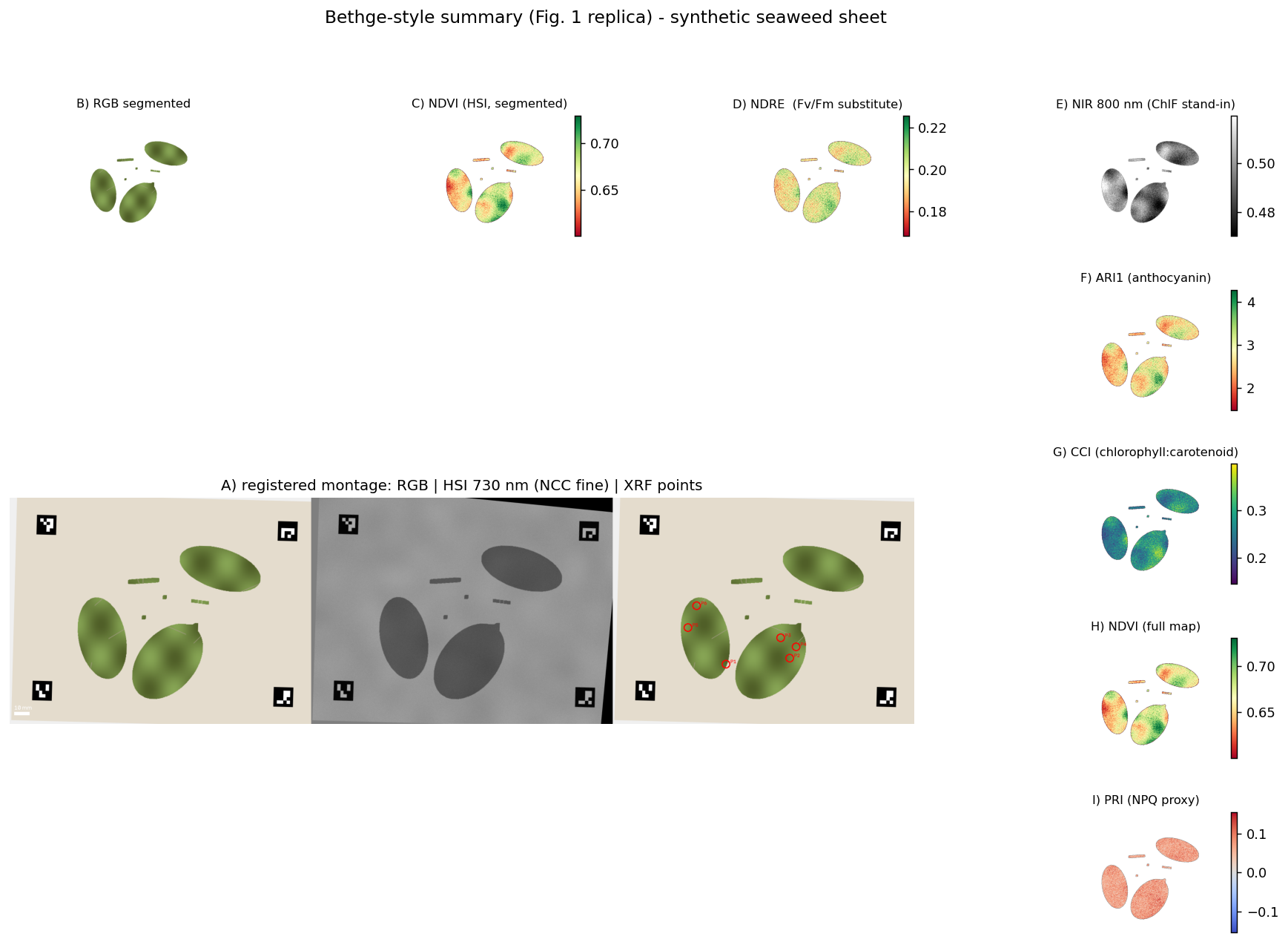
A pressed seaweed specimen is one object carrying three kinds of information: its visible morphology, its chemistry per pixel and its elemental composition. Each instrument sees that same sheet differently, with its own optics, resolution and point of view. This use case describes a complete computer vision workflow that brings the three views into one aligned coordinate system and then fuses the spectral and elemental data into better predictive models.
The complete workflow, with all 25 figures, the full technical detail and the references, is available as a downloadable PDF.
Download the full use case (PDF)
1. The Problem
A herbarium style seaweed sheet is measured with three modalities. RGB provides the visible and morphological information. NIR hyperspectral imaging provides a full reflectance spectrum at every spatial location, producing a data cube with two spatial dimensions and one spectral dimension. XRF provides elemental information at a set of discrete measurement points distributed over the sheet.
Each instrument produces an image with different spatial coordinates, because the instruments have different optics, sensor positions, resolutions and viewing geometries. The XRF instrument reports its points in sheet millimetres, the RGB camera reports pixels, and the hyperspectral scanner has its own pixel grid and its own distortions. Before any modelling is possible one question must be answered: which pixel in one image corresponds to which pixel in the others? Answering that question is the job of image registration.
Once the three views are aligned, every location on the specimen carries its morphology, its spectrum and its elemental composition, and the information can be fused and modelled together. The workflow was designed around four published methods1,2,3,4, combined into a single pipeline, with a practical layer added on top: fiducial markers and a sheet millimetre frame that let point XRF measurements be joined to hyperspectral spectra.
Everything was validated end to end on a digital sheet with known ground truth: a synthetic specimen whose true geometry, masks and element values are known exactly, so every step can be scored against the truth before touching real samples. All accuracy numbers on this page come from that validation run.
2. Step 1: Camera Calibration
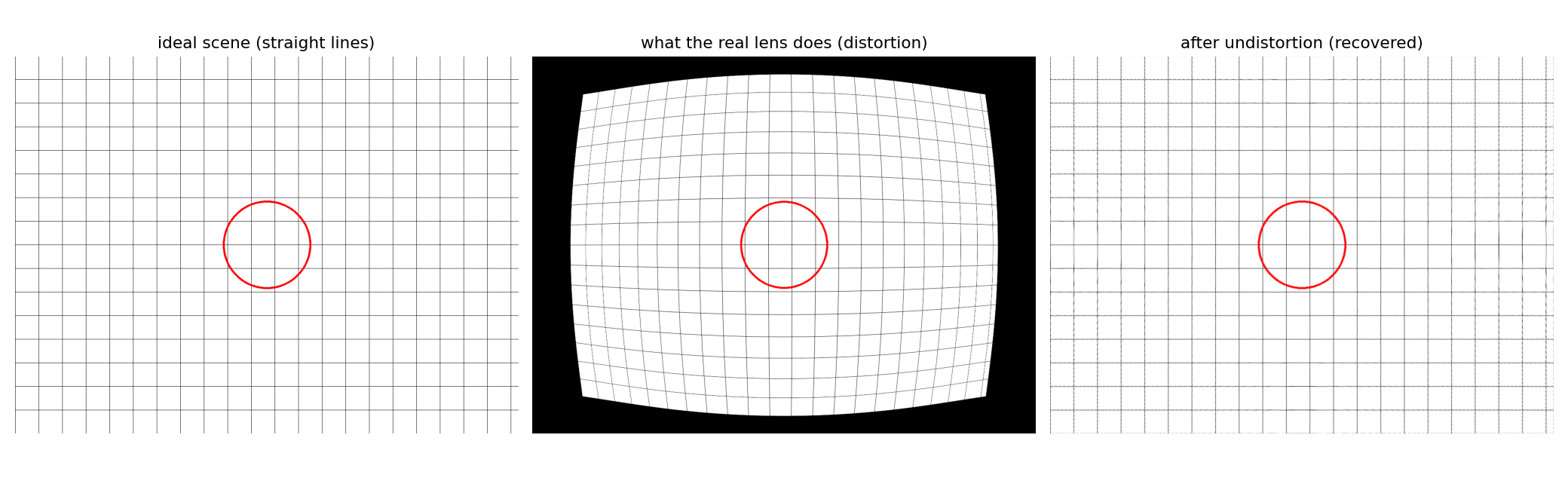
Known instrumental errors must be corrected before registration, because registration is more reliable when it works with geometrically corrected images. Cameras can have optical distortion, particularly radial distortion, in which straight lines appear slightly curved. The effect is usually stronger toward the edges of the image than near the optical centre, and it means that the same physical point may appear at slightly different pixel positions depending on where it is located in the image.
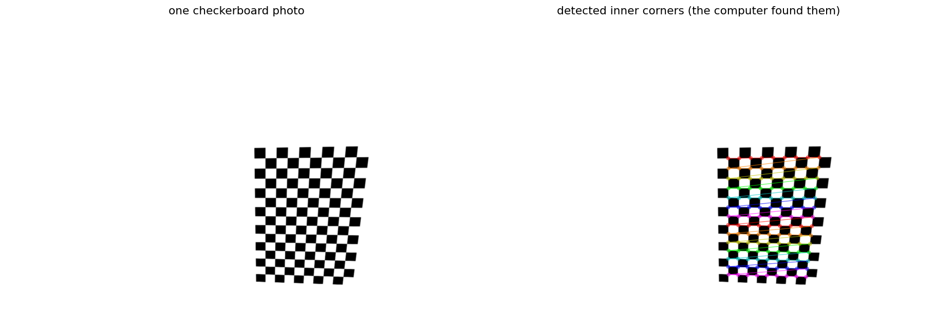
The intrinsic camera parameters are not entered manually. They are estimated mathematically during camera calibration: a checkerboard with known geometry is photographed from different positions and angles, the algorithm detects where the corners appear, and it estimates the focal lengths and the optical centre that best explain how the known 3D points of the checkerboard are projected onto the 2D image. The distortion coefficients are estimated in the same process by minimising the reprojection error. Once estimated, the pixels are remapped so the image geometry becomes closer to the real geometry of the object.
Illumination correction for the hyperspectral images. Illumination variation is caused by non uniform radiation distribution on the object plane and by changes in intensity through time. Two corrections are applied: a gradient correction, which estimates the illumination map of the image from the four corners and subtracts the unwanted pattern, and a dark and white reference normalisation, which removes the sensor dark signal and scales the result to the known reflectance factor of the reference material, 80 percent in this workflow. The goal is that differences between pixels mainly reflect real differences in the specimen rather than differences caused by uneven illumination or by the camera itself.
3. Step 2: One Coordinate System for All Modalities
One modality defines the reference coordinate system. RGB is the natural candidate here because it provides the highest spatial resolution and the clearest morphology; the hyperspectral cube and the XRF points are then transformed into the RGB coordinate system.
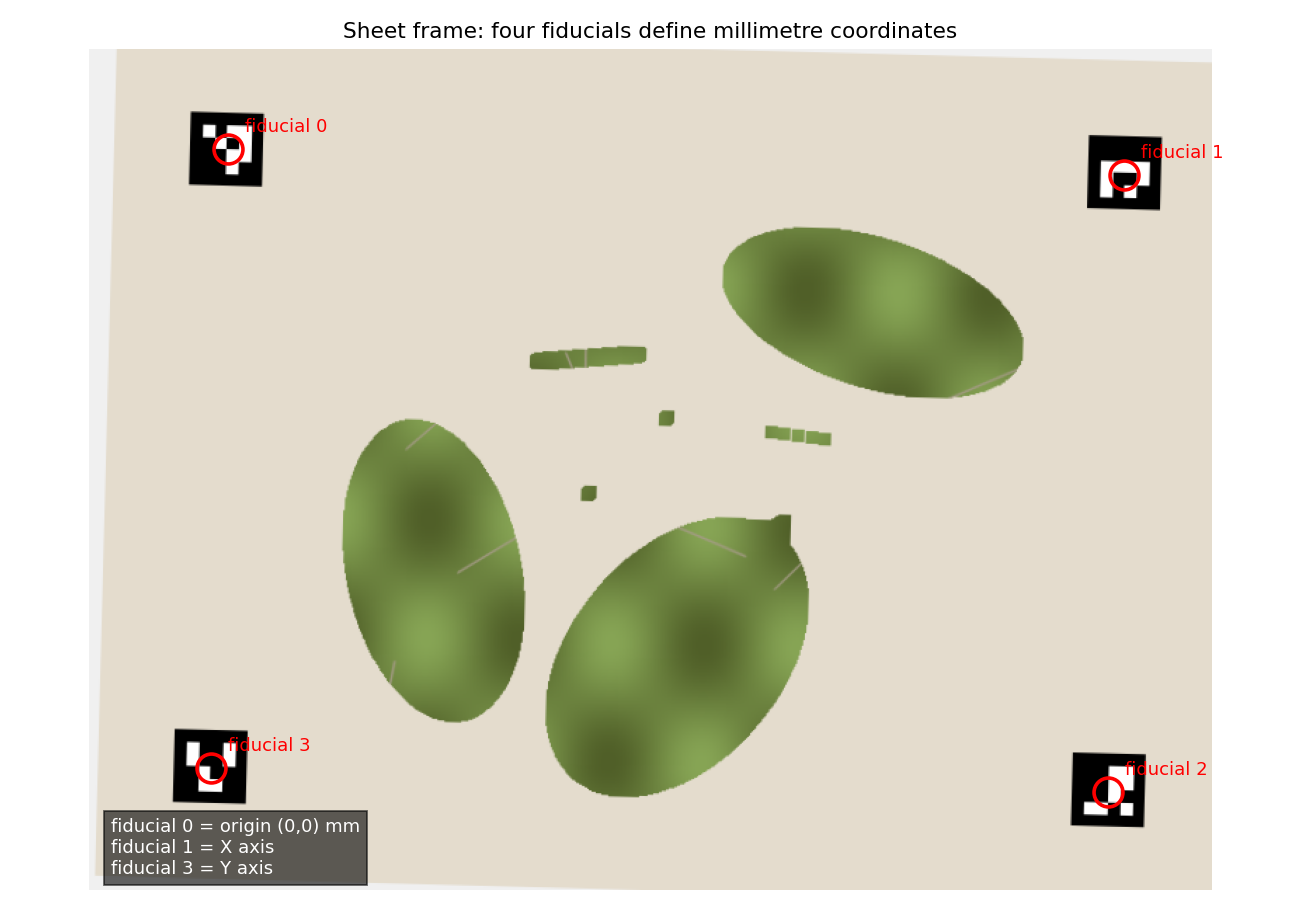
To make the mapping precise, the physical sheet carries its own frame: four ArUco fiducial markers at the corners define a millimetre coordinate system. Fiducial 0 is the origin, fiducial 1 defines the X axis and fiducial 3 defines the Y axis. Because the marker positions are known in millimetres and the markers are visible in the images, they link the real sheet, the cameras and the XRF instrument together. One golden rule applies: registration needs images that show the same object, so every sheet gets its own transformation, obtained from its own fiducials.
4. Step 3: Coarse Registration with Image Features
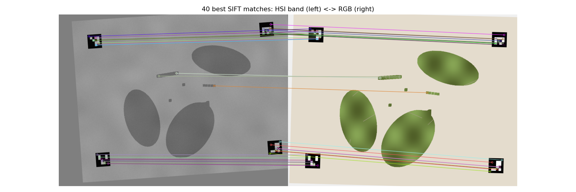
Registration means finding the transformation that makes the same physical point fall on the same pixel in two images. The coarse step gets close to the final alignment using distinctive image features: SIFT keypoints are detected in both images, a matcher pairs the points that look alike, and RANSAC finds the transformation that fits the majority of pairs while discarding the wrong ones.
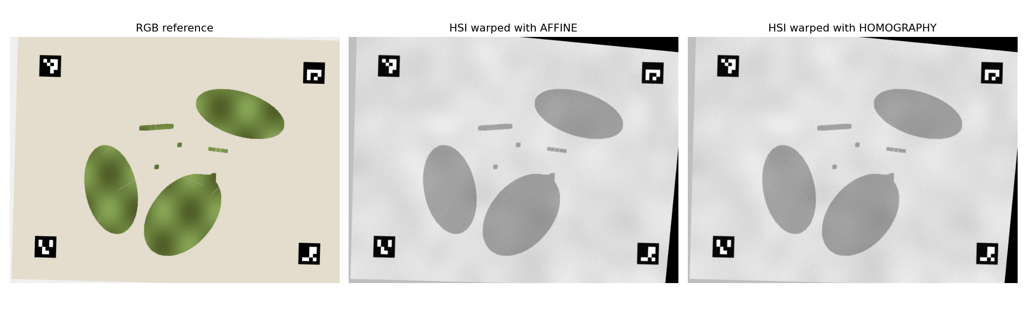
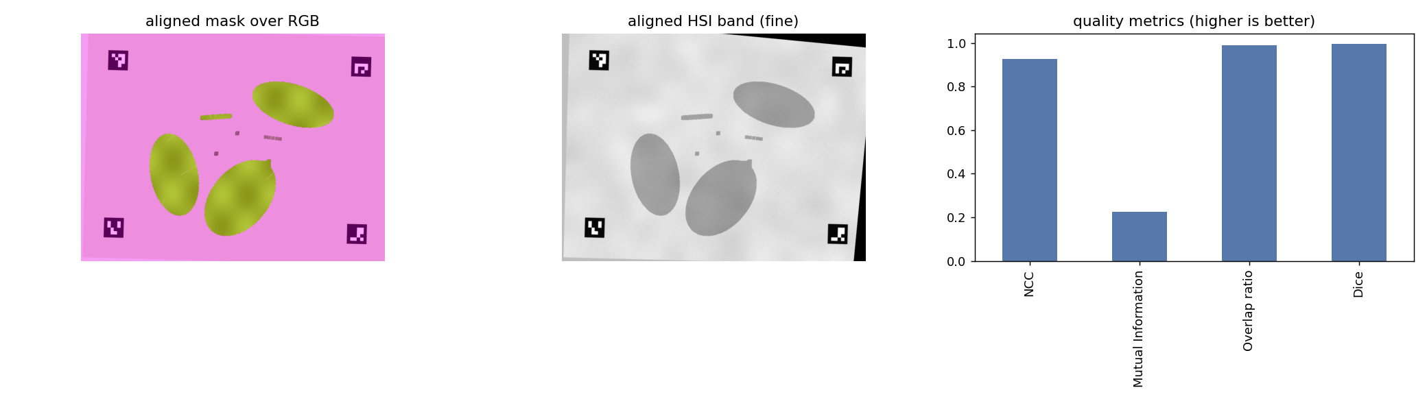
Two transformation models were estimated and compared. An affine transformation (6 parameters) can translate, rotate, scale and skew an image, and it preserves parallel lines, which suits cameras looking roughly straight at a flat object. A homography (8 parameters) additionally models perspective effects, which appear when the sensors are physically separated and observe the specimen from different viewpoints. On the validation sheet the affine model reached a landmark error of 0.80 px (NCC 0.927, Mutual Information 0.224) and the homography reached 0.79 px (NCC 0.927, Mutual Information 0.226), so the homography was selected.
The same comparison framework was used to evaluate the three registration strategies published by Rana and colleagues3: registering the complete images (A), the binary specimen masks (B) or only the pixels inside the mask (C). On this sheet the full image strategy clearly won:
The lesson is general: registration strategies must be compared on your own images instead of assumed, because the winner depends on the specimen and the background.
5. Step 4: Fine Registration with Image Intensities
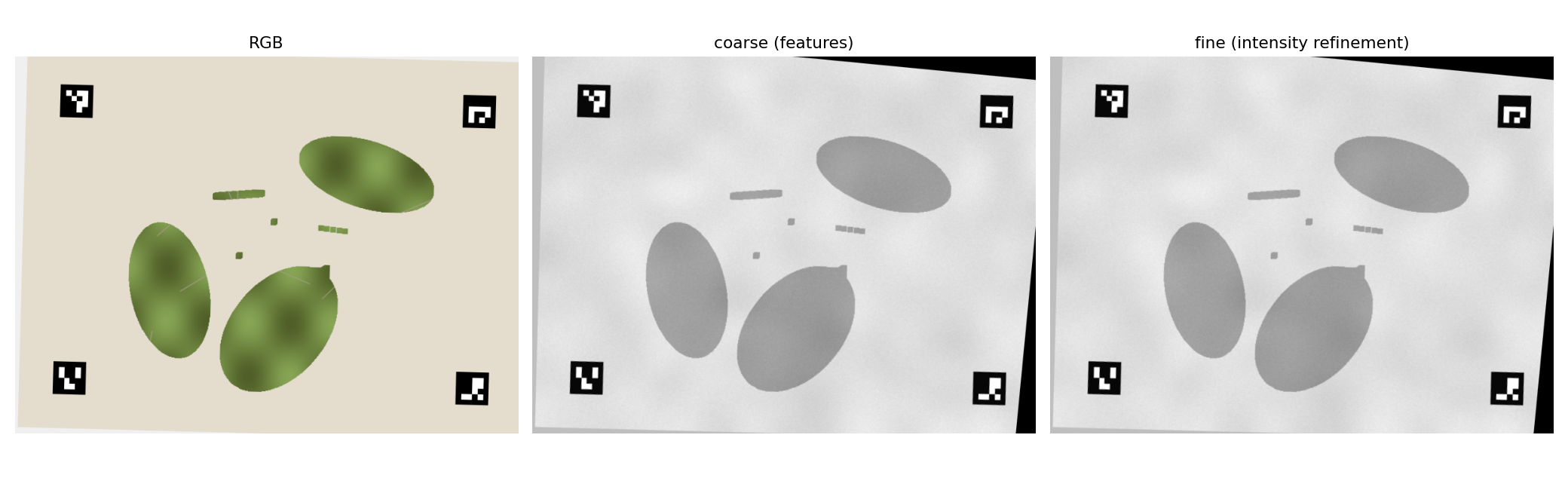
The feature based transformation is a good but not pixel perfect alignment, because features are sparse and sometimes noisy. The fine step refines it using the actual image intensities, maximising the normalised cross correlation (NCC) between the RGB reference and the warped HSI band.
For strongly multimodal pairs, Mutual Information is the metric of choice: it does not require the two images to have similar intensity values, only a statistical relationship. Starting from the coarse alignment, the algorithm makes small adjustments to the transformation and keeps searching for the one that maximises the statistical dependency between corresponding pixels, resulting in a more precise alignment. On the validation sheet the refinement brought NCC from 0.927 to 0.928 with a landmark error of 0.87 px, confirming that the coarse step was already close and the fine step corrected the remaining small misalignment.
6. Step 5: Segmentation
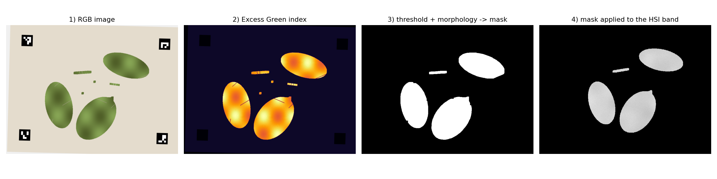
Segmentation separates the specimen from the background: paper, labels and shadows. On the RGB image an Excess Green index (2G minus R minus B) emphasises the green specimen, Otsu thresholding automatically finds the separating threshold, and morphological operations clean the binary mask by removing small isolated noise and filling small holes inside the specimen.
The hyperspectral cube offers further options, such as an NDVI computed from a near infrared band and a red band, but in this workflow the final mask is created from the RGB image because RGB provides the best spatial quality. The mask is then transferred to the registered modalities: the same spatial region identified as specimen in RGB is kept as specimen in HSI and XRF, while background pixels are excluded from the analysis. If more accuracy were needed, an automatic model such as YOLOv8 segmentation could be investigated.
7. Step 6: Did the Registration Actually Work?
The alignment is verified rather than assumed, from three angles. Geometric quality: the Overlap Ratio (how much of the specimen area coincides between the registered images), the centroid displacement (distance between the specimen centres) and the landmark error (distance between identifiable corresponding points). Multimodal quality: Mutual Information, which indicates whether the modalities contain statistically related information at corresponding locations even when the images look very different. And the failure rate: how often the algorithm produces an incorrect result. Combining geometric and multimodal metrics gives a much stronger evaluation, because a single metric may indicate good alignment while another type of error hides.
8. Step 7: Bringing the XRF Data In
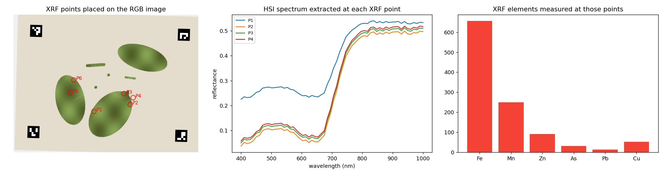
The XRF instrument reports elemental concentrations at discrete points in sheet millimetres, together with the beam footprint and the positioning uncertainty. It has no lens and therefore no lens distortion; its calibration is the energy calibration of Step 1 plus the geometric registration of its measurement points to the sheet frame.
The join works through the fiducials: the four corner markers, known in millimetres on the sheet and detected in pixels in the images, define the mapping from sheet millimetres to image pixels. Every XRF point is mapped into the registered images, and around each point a circular region of interest is extracted with a radius that covers the beam diameter plus the positioning uncertainty. Inside each region the mean NIR reflectance spectrum is extracted from the cube. The result is a joined table with one row per XRF point: sheet coordinates, pixel coordinates, elemental concentrations and the full NIR spectrum at that location. On the validation sheet the mean position error of the mapped points was 0.84 px (maximum 1.30 px), and the extracted spectra matched the ground truth with r = 1.000.
9. Step 8: Data Fusion and Model Evaluation
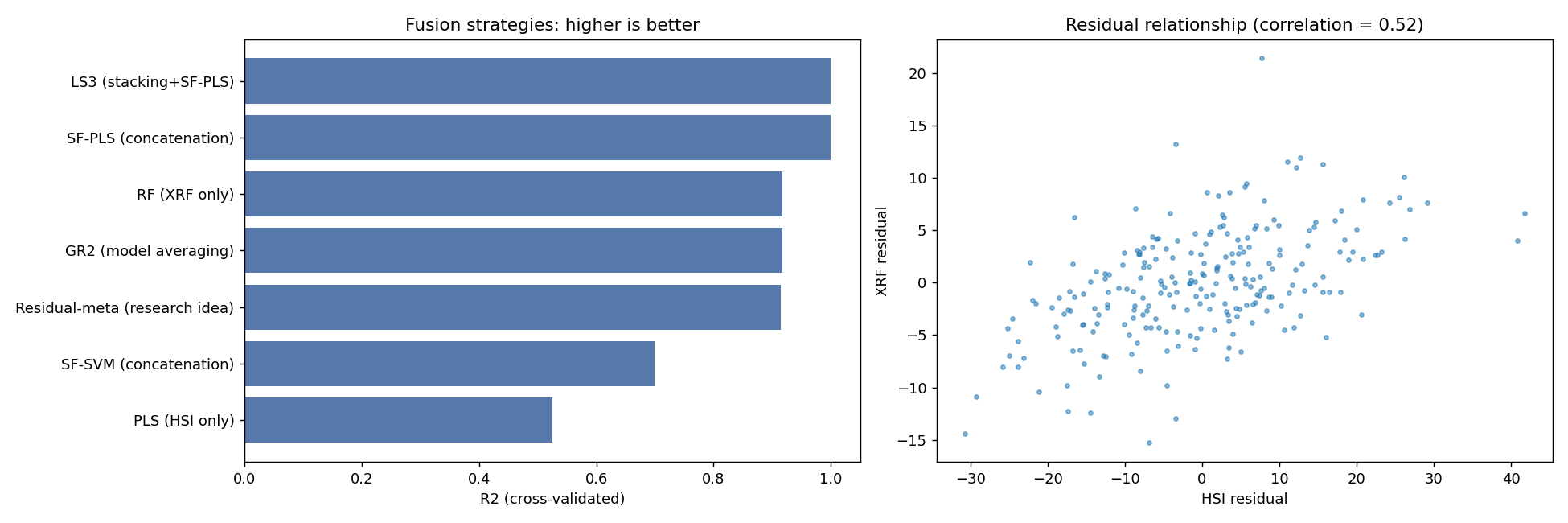
Once spectra and elements are aligned, the fusion strategies were compared systematically rather than assumed4. In early fusion the spectral variables and the elemental concentrations are concatenated into one combined dataset that feeds a single predictive model. In model level fusion each sensor gets its own model, and the separate predictions are combined by model averaging (GR2) or by stacking (LS3). The least squares combination also considers the covariance between the prediction residuals: if the individual sensor models tend to make correlated errors, that shared structure can be exploited when combining their predictions. A residual structure meta model was additionally explored, feeding the difference between the two model residuals and a local residual correlation into a meta learner.
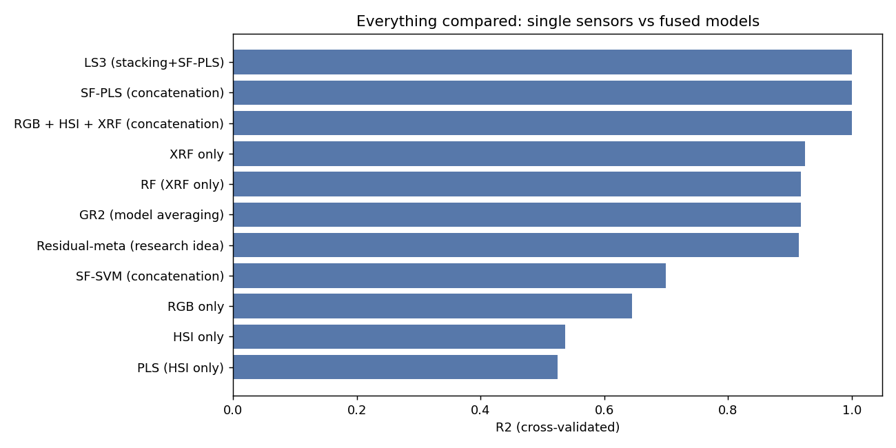
On the validation cohort (cross validated), the spectra alone reached R² 0.525 (PLS) and the elements alone R² 0.918 (random forest). The fused models clearly outperformed both single sensor models:
The final question is not only which model has the lowest error, but what information each modality contributes, when multimodal integration improves the result, and whether that improvement has a biological interpretation. On real specimens the ranking must be re measured with nested, per specimen cross validation.
10. Real Data Behind Every Stage
No public dataset combines RGB, hyperspectral and XRF measurements of the same object, so each stage is validated against real data of its own while the end to end behaviour is proven on the synthetic ground truth sheet. The XRF side follows the published protocol for elemental analysis of herbarium sheets with portable EDXRF, including cardboard backing controls, adhesive considerations and the treatment of overlapping emission peaks.
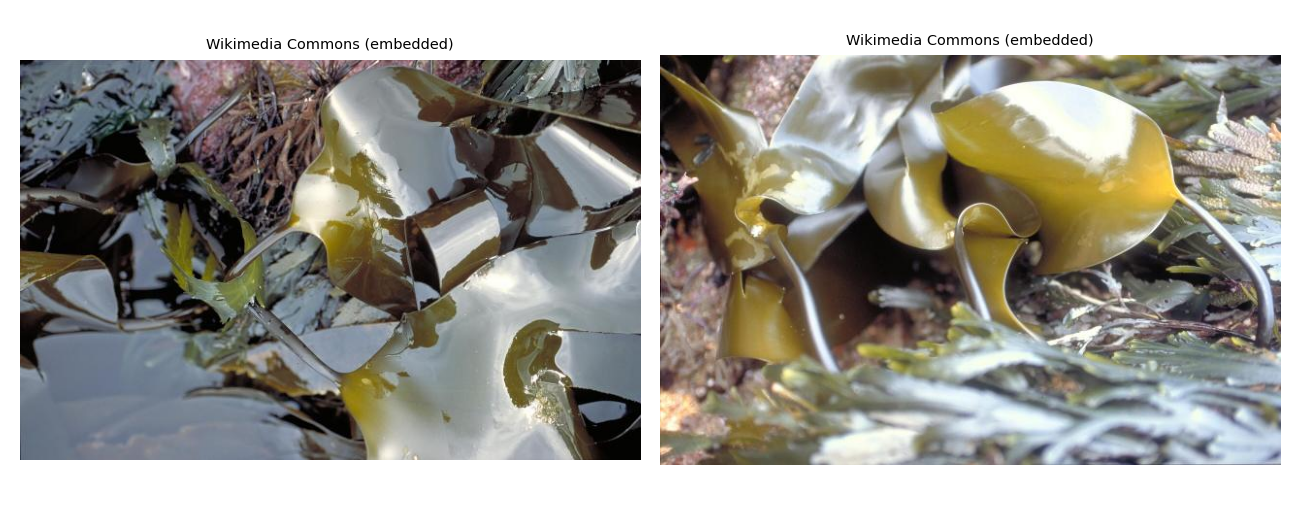
Already integrated in the pipeline loaders: real portable EDXRF tables from ten macroalgae samples (13 elements each), published element concentrations across ten seaweed species from Greenland (17 elements)5, real reflectance spectra from the GLORIA water quality dataset6 and real hyperspectral root images from the HyperPRI dataset7, used to test the calibration and registration path on measured camera data. The downloadable PDF expands this section with those figures.
11. What This Workflow Delivers
- One sheet frame: morphology, spectrum and elements referred to the same physical point, with sub pixel accuracy (landmark error 0.87 px, overlap 0.99).
- Measured quality: every step reports its own metrics, from the calibration reprojection error to cross validated R2, so quality is verified instead of assumed.
- Better models through fusion: in the validation cohort, the fused spectral and elemental models clearly outperformed both single sensor models.
- Instrument agnostic: the workflow works with pressed and flat specimens of any kind where image, spectrum and chemistry must be brought together.
Vibralytics provides research services, custom pipelines and training for exactly this type of multimodal imaging and chemometrics work. If your laboratory or collection needs to combine cameras, hyperspectral imaging and elemental analysis, talk to us.
Download the full use case (PDF) Contact us
12. References
- Bethge HL, et al. Automated image registration of RGB, hyperspectral and chlorophyll fluorescence imaging data. Plant Methods. 2024. Available from: Plant Methods 2024
- Sharma N, et al. An Open-Source Package for Thermal and Multispectral Image Analysis for Plants in Glasshouse. Plants. 2023. Available from: Plants 2023
- Rana S, et al. Comprehensive Evaluation of Multispectral Image Registration Strategies in Heterogenous Agriculture Environment. J Imaging. 2024. Available from: J Imaging 2024
- Tavares TR, et al. Combined Use of Vis-NIR and XRF Sensors for Tropical Soil Fertility Analysis: Assessing Different Data Fusion Approaches. Sensors. 2020. Available from: Sensors 2020
- Kreissig KJ, et al. Characterisation and chemometric evaluation of 17 elements in ten seaweed species from Greenland. PLOS ONE. 2021. Available from: PLOS ONE 2021
- Lehmann MK, et al. GLORIA: a global dataset of remote sensing reflectance and water quality from inland and coastal waters. PANGAEA. 2022. Available from: PANGAEA 2022
- Chang SJ, et al. HyperPRI: a dataset of hyperspectral images for underground plant root study. Computers and Electronics in Agriculture. 2024. Available from: Comput Electron Agric 2024
- Seaweed photographs from Wikimedia Commons, free licences. Portable EDXRF macroalgae dataset: own measurements, ten samples by 13 elements.